Discovering the Beauty of Implicit Equations
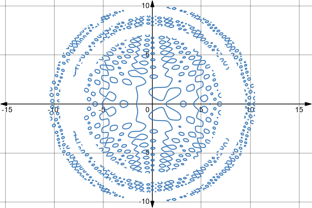
Dear readers and math lovers! Today I’m excited to share with you my entry in a very special contest organised by Mates Mike, a content creator who teaches mathematics through animations. The challenge is to find an implicit equation \(F(x, y) = 0\) with a surprising graph. I see this as the perfect opportunity to explore and share the fascinating world of the graphs generated by implicit equations and implicit functions.
In this article I’ll take you on a journey of discovery, where we will explore several techniques and properties for creating fascinating graphs with implicit equations. As we go, I’ll unveil the secrets and the concepts I learned throughout the contest. I hope you find inspiration and enjoy this experience as much as I did!
Introduction to implicit equations and functions
What is an implicit equation?
An implicit equation is a relation of the form \(F(x_1, \dots, x_n) = 0\) where \(F\) is a function of the variables \(x_1, \dots, x_n\). The locus, on the other hand, is the set of points \(P(x_1, \dots, x_n)\) of \(\mathbb{R}^n\) that satisfy the implicit equation \(F\).
The locus of an implicit equation is simply its graph.
For instance, let’s think about the two-variable implicit equation
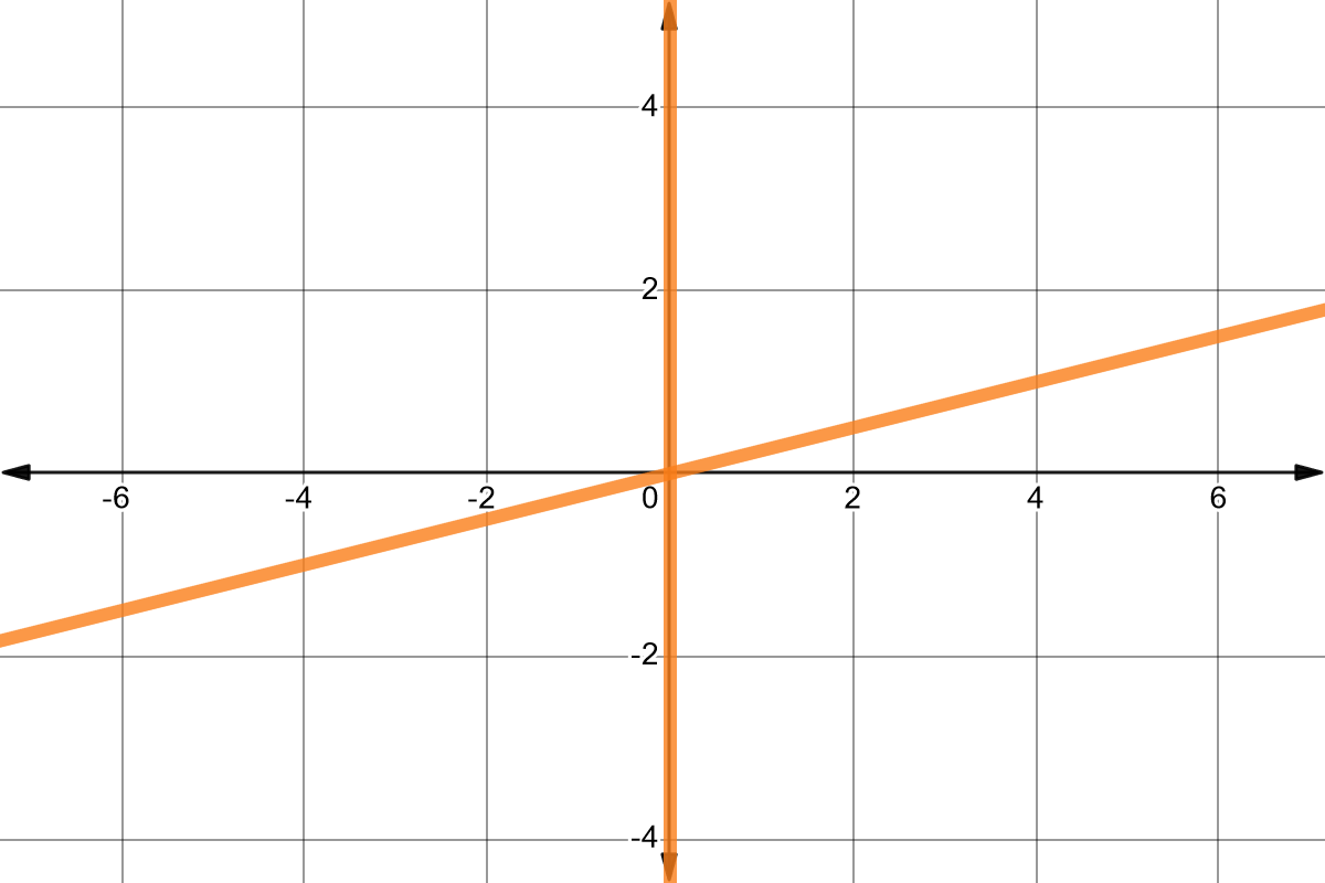
\[F(x, y) = x^2 - 4xy = 0\]What kind of locus does it represent? Put another way, which curve do the points satisfying this equation determine? If we factor out \(x\) we get:
\[x(x-4y) = 0\]Therefore, the points satisfying the implicit equation \(F(x, y) = 0\) are the points of the line \(x = 0\) and the points of the line \(x = 4y\).
We can plot this locus in Desmos:
What is an implicit function?
An implicit function is a function defined by an implicit equation, and it relates one of the variables, called the dependent variable, to the remaining ones, called the independent variables.
\[F(x, y) = 0 \iff y = f(x)\]The main difference between an implicit equation and an implicit function is that the implicit equation does not distinguish between independent and dependent variables, whereas the implicit function does. We can say that every implicit function is an implicit equation, while not every implicit equation is an implicit function.
In general, an implicit equation has multiple implicit functions if, when solving for \(y\), we reach a step where we have to make a choice, such as a square root. For example, consider the implicit equation \(y^2 - x = 0\). Solving for \(y\) we get:
\[y^2 = x\] \[y = \pm \sqrt{x}\]Therefore, this implicit equation is defined by two implicit functions:
\[y_1 = \sqrt{x} \quad \land \quad y_2 = -\sqrt{x}\]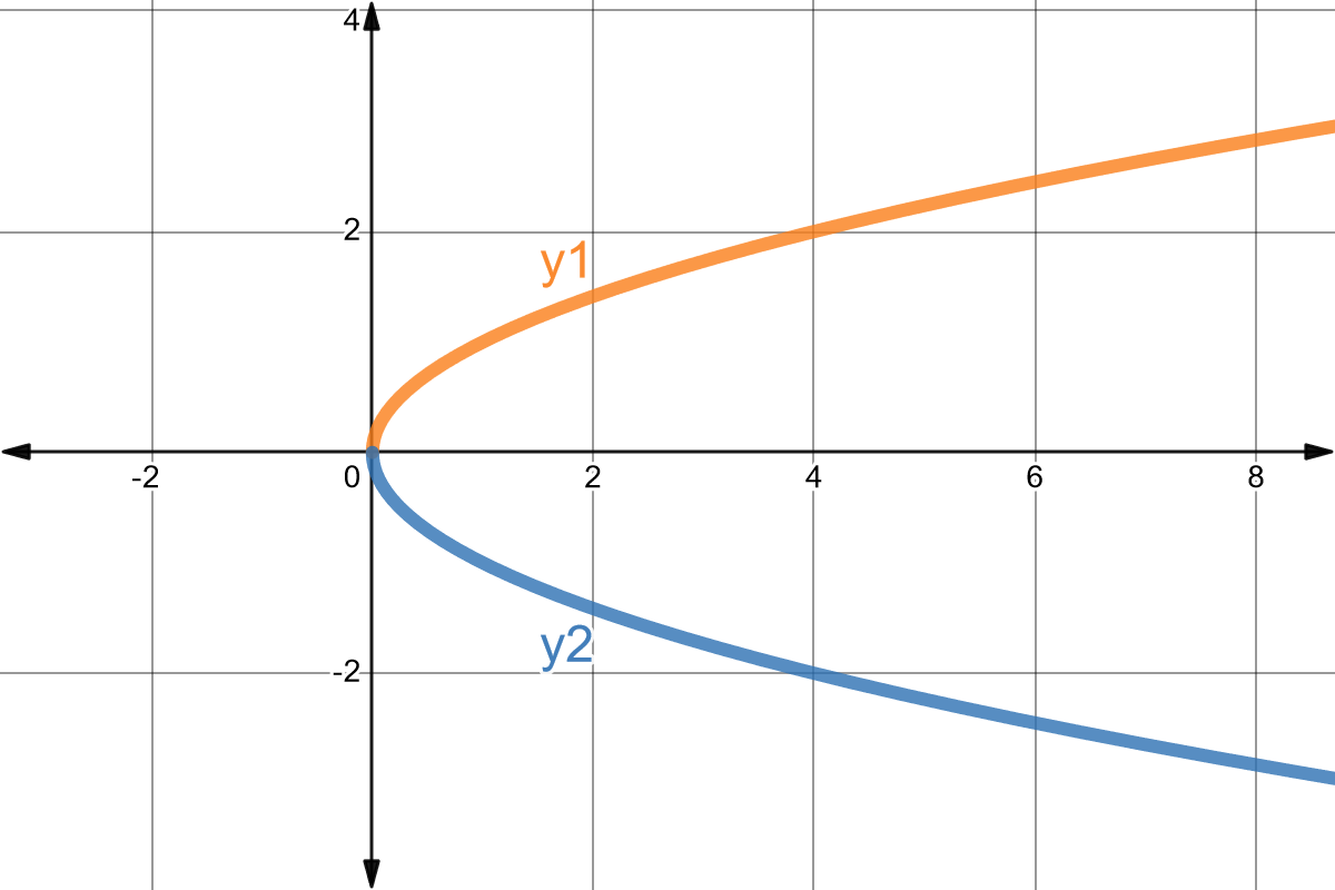
Implicit equation of the circle
A circle is the locus formed by the set of all the points of a plane that are equidistant from a fixed point \(C\) called the centre. The distance from any point \(P\) of the circle to the centre \(C\) is called the radius and is denoted by \(r\).
Let \(P(x, y)\) be any point of the circle whose centre is \(C(a, b)\) and whose radius measures \(r\). Then, by the definition of a circle, \(d(P, C)=r\); that is, the Euclidean distance between the centre of the circle and any of its points equals the radius.
\[d(P, C) = r \iff \sqrt{(x - a)^2 + (y - b)^2} = r\]From which it follows that:
\[(x - a)^2 + (y - b)^2 = r^2\]This is the implicit equation of the circle of radius \(r\) and centre \((a, b)\), and the locus of the circle is:
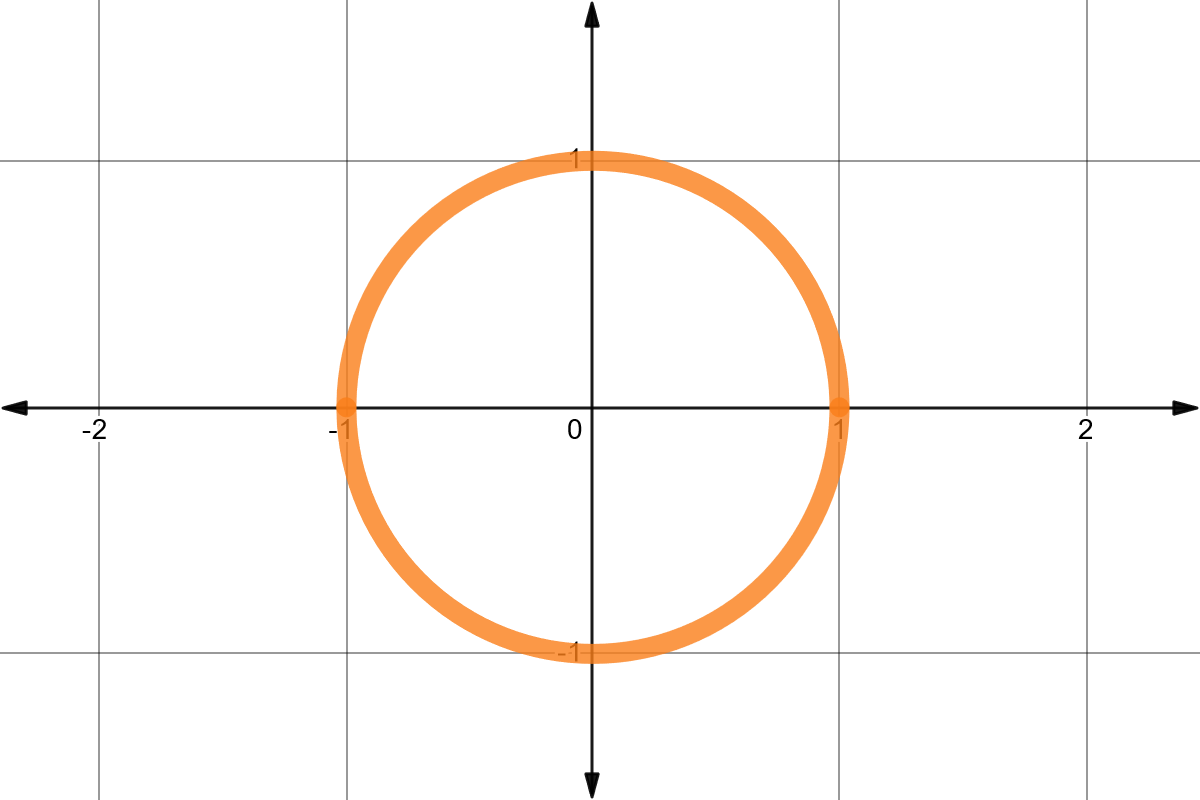
\[\{(x, y) \in \mathbb{R}^2 \mid (x - a)^2 + (y - b)^2 = r^2\}\]Let’s take the example of a circle centred at the origin with radius \(r = 1\). Its implicit equation is:
\[x^2 + y^2 = 1\]And its locus is:
Properties of implicit equations
Below we will look at several properties of implicit equations that let us translate, expand, compress, reflect and combine different loci. This way we can transform any graph we like to create surprising new graphs with great ease.
Translation
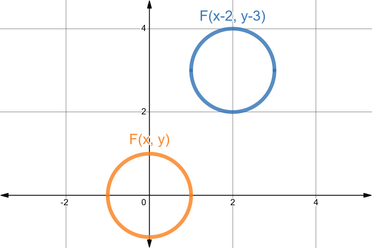
With this property we can move our graphs across the plane. Given an implicit equation \(F(x, y) = 0\), the locus of \(F\) translated \(a\) units along the \(x\) axis and \(b\) units along the \(y\) axis is defined by the implicit equation:
\[F(x - a, y - b) = 0\]Proof
We can prove the translation easily by considering the substitution variables \(u = x-a\) and \(v = y-b\), so that \(F(x-a, y-b) = F(u, v)\). Let \(P(u, v) = (x_0, y_0)\) be any point belonging to the locus of \(F(u, v) = 0\); we can observe that:
\[\begin{align*} P(u, v) &= (x_0, y_0) \\ P(x-a, y-b) &= (x_0, y_0) \\ P((x-a) + a, (y-b) + b) &= (x_0 + a, y_0 + b) \\ \therefore P(x, y) &= (x_0 + a, y_0 + b) \end{align*}\]Example
As an example, let’s consider a unit circle of radius \(1\) centred at the origin. Its implicit equation is \(F(x, y) = x^2 + y^2 - 1 = 0\). If we translate the circle \(2\) units along the \(x\) axis and \(3\) units along the \(y\) axis, the implicit equation of the translated circle is:
\[F(x-2, y-3) = (x-2)^2 + (y-3)^2 - 1 = 0\]And its locus is:
Expansion, compression and reflection
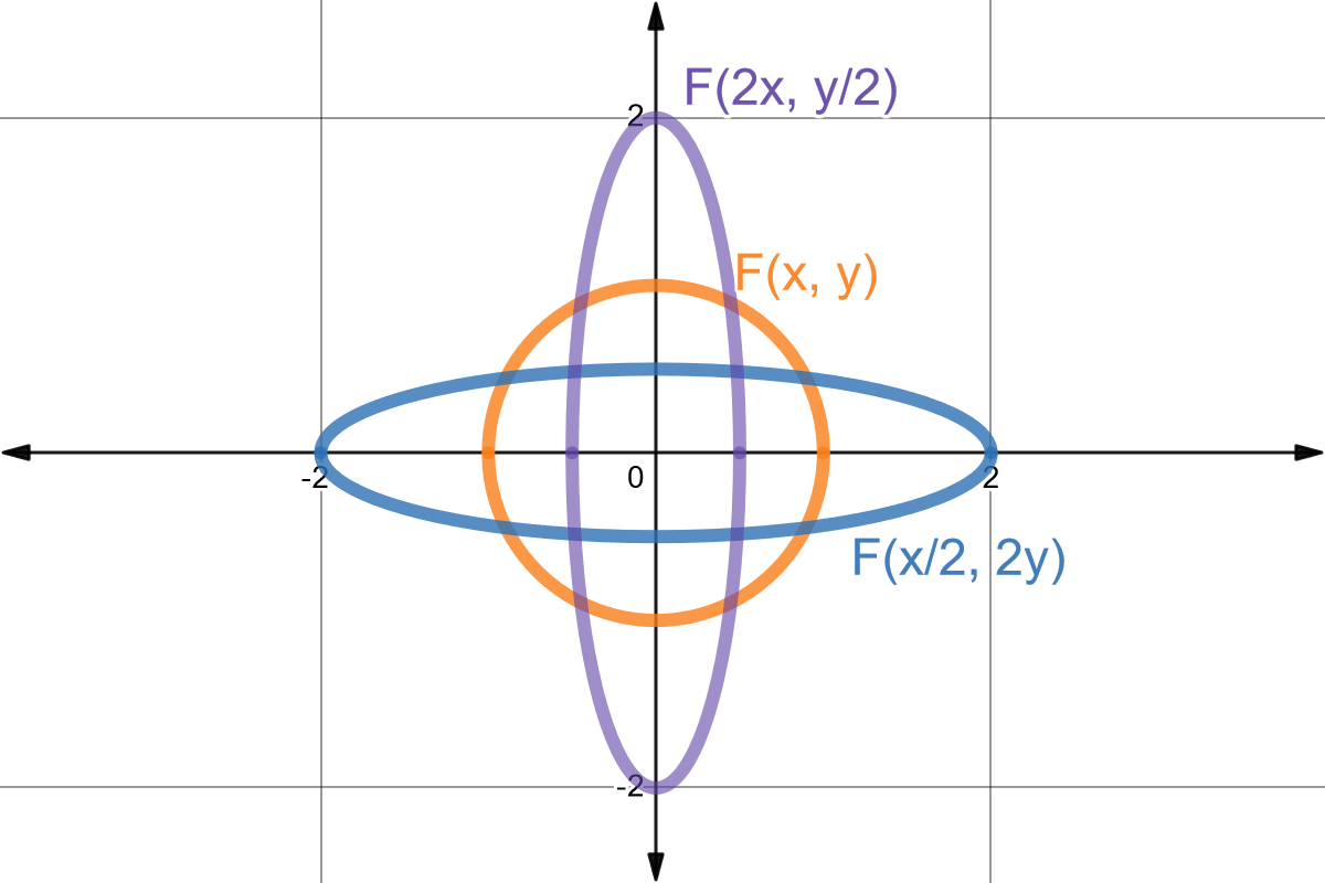
The following property lets us stretch, shrink and flip our graphs with respect to the different axes. Given \(F(x, y) = 0\), the implicit equation of the same curve expanded, compressed and/or reflected by \(a\) units along the \(x\) axis and \(b\) units along the \(y\) axis is:
\[F(a x, b y) = 0\]Where if:
- \(0 < \|a\| < 1\): expansion with respect to the \(x\) axis.
- \(\|a\| > 1\): contraction with respect to the \(x\) axis.
- \(a < 0\): reflection with respect to the \(y\) axis.
- \(0 < \|b\| < 1\): expansion with respect to the \(y\) axis.
- \(\|b\| > 1\): contraction with respect to the \(y\) axis.
- \(b < 0\): reflection with respect to the \(x\) axis.
Note that a negative value of \(a\) produces a reflection about the \(y\) axis and not about the \(x\) axis, just as a negative value of \(b\) produces a reflection about the \(x\) axis.
Proof
To prove this we follow the same procedure used for the translation property. We define the substitution variables \(u = a x\) and \(v = b y\), so that \(F(a x, b y) = F(u, v)\), and take any point \(P(u, v) = (x_0, y_0)\) belonging to the locus of \(F(u, v) = 0\):
\[\begin{align*} P(u, v) &= (x_0, y_0) \\ P(a x, b y) &= (x_0, y_0) \\ P(\frac{a x}{a}, \frac{b y}{b}) &= (\frac{x_0}{a}, \frac{y_0}{b}) \\ \therefore P(x, y) &= (\frac{x_0}{a}, \frac{y_0}{b}) \end{align*}\]Example
Given the implicit equation of the unit circle \(F(x, y) = x^2 + y^2 - 1 = 0\), we can find the circle expanded twofold with respect to the \(x\) axis and compressed by half with respect to the \(y\) axis, \(F(\frac{1}{2}x, 2y)\); and the circle compressed by half with respect to the \(x\) axis and expanded twofold with respect to the \(y\) axis, \(F(2x, \frac{1}{2}y)\).
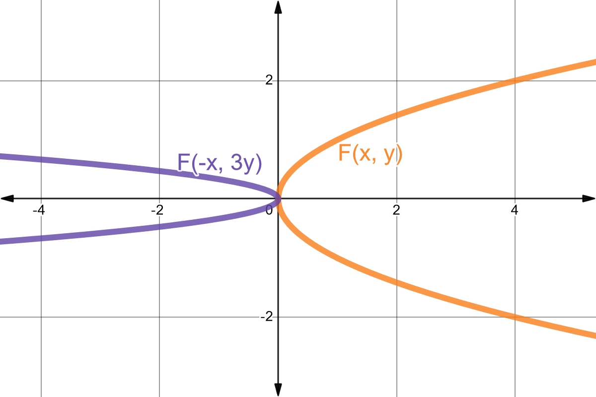
Now let’s take the implicit equation of the parabola \(G(x, y) = y^2 - x = 0\) and observe how the implicit equation \(G(-x, 3y)=0\) is the same parabola, but reflected about the \(y\) axis and compressed threefold along that same axis.
Union
This property lets us join several graphs into a bigger one, which is very interesting when we want to bring together two loci of our choosing. Given two implicit equations \(F(x, y)=0\) and \(G(x, y)=0\), the implicit equation whose locus is the union of the loci of \(F\) and \(G\) is:
\[F(x, y) \cdot G(x, y) = 0\]Proof
To prove the union property, simply note that:
\[F(x, y) \cdot G(x, y) = 0 \iff F(x, y) = 0 \lor G(x, y) = 0\]So the locus \(D\) of \(F(x, y) \cdot G(x, y) = 0\) is:
\[\begin{align*} D &= \{(x, y) \in \mathbb{R}^2 \mid F(x, y) = 0\} \quad \cup \quad \{(x, y) \in \mathbb{R}^2 \mid G(x, y) = 0\} \\ \therefore D &= \{(x, y) \in \mathbb{R}^2 \mid F(x, y) = 0 \lor G(x, y) = 0\} \end{align*}\]Example
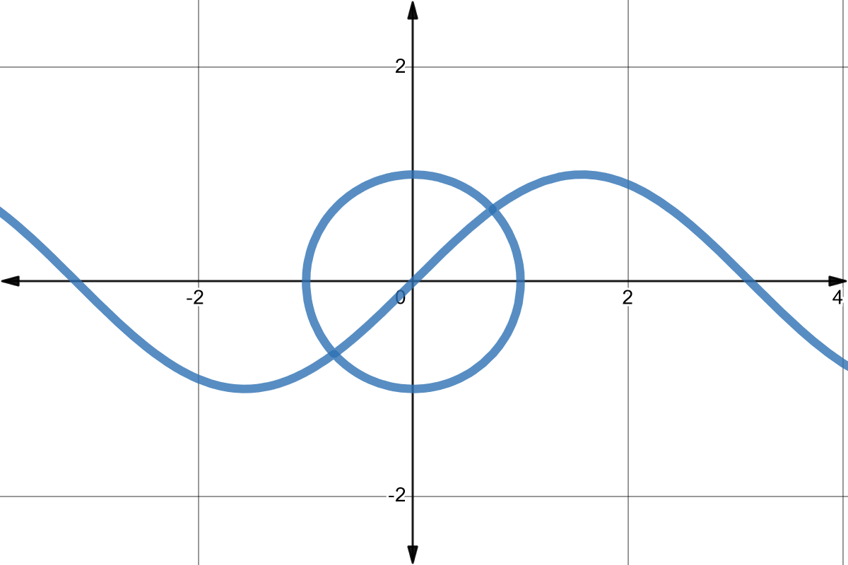
Let’s take the example of the implicit function of the sine \(F(x, y) = y - \sin{x} = 0\) and the implicit equation of the unit circle centred at the origin \(G(x, y) = x^2 + y^2 - 1 = 0\).
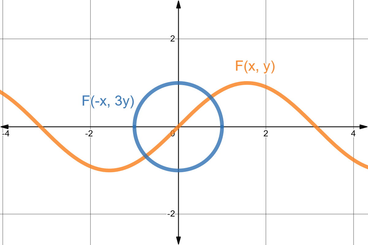
If we apply the union property to \(F\) and \(G\) we get the implicit equation:
\[F(x, y) \cdot G(x, y) = (y - \sin{x}) \cdot (x^2 + y^2 - 1) = 0\]whose locus is the combination of the loci of \(F\) and \(G\):
Reduction of loci
We call reduction of loci the technique by which some points are removed from the locus of an implicit equation. This lets us combine loci in many ways, greatly widening the range of graphs we can create.
Definition
Given an implicit equation \(F(x_1, \dots, x_n) = 0\) with locus \(D_F\), we define the reduced equation \(F'(x_1, \dots, x_n) = 0\) with locus \(D_{F'}\), where
\[D_{F'} \subseteq D_{F}\]and the reduction function \(\Phi : \mathbb{R}^n - R \rightarrow \{1\}\) such that
\[F'(x_1, \dots, x_n) = F(x_1, \dots, x_n) \cdot \Phi(x_1, \dots, x_n)\]where \(R\) is the reduction set containing the points we want to remove from the locus of \(F(x_1, \dots, x_n) = 0\). In this way, the locus of \(F'(x_1, \dots, x_n) = 0\) is determined as
\[D_{F'} = \{(x_1, \dots, x_n) \in \mathbb{R}^n \mid F(x_1, \dots, x_n) = 0 \land (x_1, \dots, x_n) \notin R\}\]Explanation
The idea is to find a way to remove a set of points \(R\) from the locus defined by the implicit function \(F(x_1, \dots, x_n) = 0\). To do so we look for a reduction function \(\Phi\) that returns \(1\) for any value of \(x_1, x_2, \dots, x_n\), but whose domain is restricted by \(R\), so that \(F(x_1, \dots, x_n) \cdot \Phi = F(x_1, \dots, x_n)\) for every point of \(D_F\) except those values that lie in \(R\). This way, the locus of the reduced implicit equation \(D_{F'}\) is determined by all the points belonging to \(D_F\) minus those that also belong to \(R\), that is:
\[D_{F'} = D_F - R\]To achieve this we use certain mathematical indeterminacies, such as division by zero and the square root of negative numbers, as will be analysed in more detail in the following sections.
Reduction by distinction
Goal
Reduction by distinction lets us remove the points of a locus that also belong to another locus. That is, given the implicit equations \(F(x_1, \dots, x_n) = 0\) and \(G(x_1, \dots, x_n) = 0\), we want to remove from the locus of \(F\) those points that also satisfy the implicit equation of \(G\). The reduction set \(R\) is then:
\[R = D_F - D_G\]where \(D_F\) is the locus of \(F\) and \(D_G\) is the locus of \(G\).
Reduction function
Given the implicit equations \(F(x_1, \dots, x_n) = 0\) and \(G(x_1, \dots, x_n) = 0\), we define the reduction function \(\Phi(x_1, \dots, x_n)\) as
\[\Phi(x_1, \dots, x_n) = \frac{G(x_1, \dots, x_n)}{G(x_1, \dots, x_n)}\]so that
\[F'(x_1, \dots, x_n) = F(x_1, \dots, x_n) \cdot \frac{G(x_1, \dots, x_n)}{G(x_1, \dots, x_n)}\]with locus equal to
\[D_F' = \{(x_1, \dots, x_n) \in \mathbb{R}^n \mid F(x_1, \dots, x_n) = 0 \land G(x_1, \dots, x_n) \neq 0\}\]Reduction by inequality
Goal
With reduction by inequality we want to remove the points of a locus that satisfy a given less than or equal inequality. Consider the implicit equation \(F(x_1, \dots, x_n) = 0\) and the inequality \(G(x_1, \dots, x_n) \leq 0\); we want to remove from the locus \(D_F\) those points that satisfy the inequality. The reduction set \(R\) is defined as:
\[R = D_F - \{(x_1, \dots, x_n) \in \mathbb{R}^n \mid G(x_1, \dots, x_n) \leq 0\}\]where \(D_F\) is the locus of \(F\).
Reduction function
Given the implicit equation \(F(x_1, \dots, x_n) = 0\) and the inequality \(G(x_1, \dots, x_n) \leq 0\), we define the reduction function \(\Phi(x_1, \dots, x_n)\) as
\[\Phi(x_1, \dots, x_n) = \frac{\sqrt{G(x_1, \dots, x_n)}}{\sqrt{G(x_1, \dots, x_n)}}\]so that
\[F'(x_1, \dots, x_n) = F(x_1, \dots, x_n) \cdot \frac{\sqrt{G(x_1, \dots, x_n)}}{\sqrt{G(x_1, \dots, x_n)}}\]with locus equal to
\[D_F' = \{(x_1, \dots, x_n) \in \mathbb{R}^n \mid F(x_1, \dots, x_n) = 0 \land G(x_1, \dots, x_n) > 0\}\]Corollary of the reduction by inequality
We can remove the points of a locus that satisfy a given greater than or equal inequality. To do so, let’s consider the implicit equation \(F(x_1, \dots, x_n) = 0\) and the inequality \(M(x_1, \dots, x_n) \leq 0\) where
\[M(x_1, \dots, x_n) = -G(x_1, \dots, x_n)\]This gives us the inequality \(M(x_1, \dots, x_n) \leq 0\), which is equivalent to the inequality \(G(x_1, \dots, x_n) \geq 0\), and the reduction function is
\[\Phi(x_1, \dots, x_n) = \frac{\sqrt{-G(x_1, \dots, x_n)}}{\sqrt{-G(x_1, \dots, x_n)}}\]Example
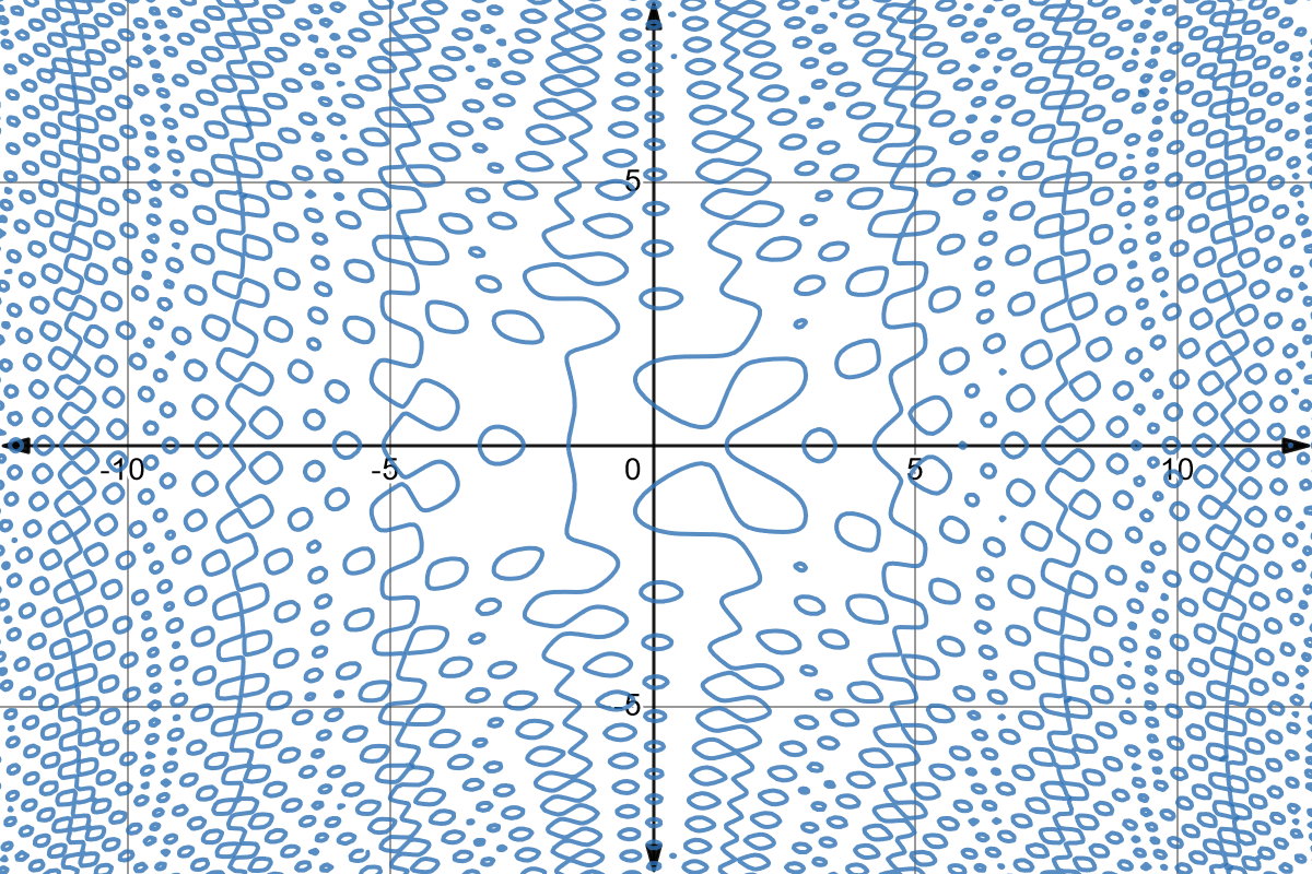
Let’s consider the implicit equation \(F(x, y) = \cos\left(x+\cos\left(yx\right)-\sin\left(x^{2}-y^{2}\right)\right)=0\), which generates this incredible locus:
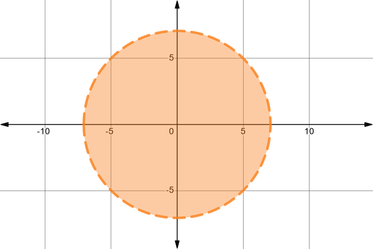
and the inequality of the circle of radius \(\sqrt{50}\) centred at the origin, \(G(x,y)=x^{2}+y^{2}-50<0\):
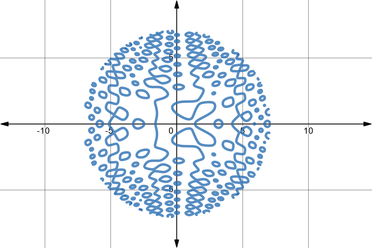
Using the corollary of the reduction by inequality we can plot only the portion of the locus of \(F(x, y) = 0\) that lies inside the circle \(G(x,y)=0\). To do so we define the reduced implicit equation
\[F'(x, y) = F(x, y) \cdot \Phi(x, y) = F(x, y) \cdot \frac{\sqrt{-G(x,y)}}{\sqrt{-G(x,y)}} = 0\]and by substituting we get
\[F'(x, y) = \cos\left(x+\cos\left(yx\right)-\sin\left(x^{2}-y^{2}\right)\right) \cdot \frac{\sqrt{50-x^{2}-y^{2}}}{\sqrt{50-x^{2}-y^{2}}} = 0\]We can now look at the fascinating graph generated by \(F'(x, y) = 0\):
Building a surprising graph
After going through the properties of implicit equations and learning how to play with loci, we have at our disposal a broad set of tools for building a surprising graph.
A proposed strategy
When building a graph it helps to follow a solid strategy that lets us take advantage of the properties of implicit equations effectively. Here is a series of steps for creating your own surprising graph:
Define the background of the graph: the first step is to choose an implicit equation \(F(x, y) = 0\) whose locus will act as the background of the graph. This implicit equation should represent an interesting shape or a pattern that we want to highlight in our graph.
Determine the desired shape: next, we have to define the shape our graph will take. This means defining an implicit equation \(G(x, y)=0\) containing interesting curves, such as circles, ellipses, hyperbolas or other more complex curves.
Explore and adjust: it is important to explore different options and adjust the parameters of the implicit equations to obtain the graph we want. We can experiment with translations, expansions, compressions, reflections and unions to achieve interesting visual effects.
Combine the implicit equations: once we have the implicit equation \(F(x, y) = 0\) as the background of the graph and the implicit equation \(G(x, y) = 0\) as the desired shape, we combine both equations through a reduction of loci. This produces a final implicit equation \(M(x, y) = 0\) representing our final result.
By following this strategy we can build a surprising graph by combining the background of the graph with a desired shape using the reduction of loci technique. Creativity and experimentation play a key role in this process, so don’t hesitate to try different ideas and adjustments to reach the result you want. Below you will find the construction process of the fascinating graph shown in the introduction.
Defining the background of the graph
For the background of our graph we will use the implicit equation introduced in the example of the corollary of the reduction by inequality.
\[F(x, y) = \cos\left(x+\cos\left(yx\right)-\sin\left(x^{2}-y^{2}\right)\right)=0\]whose locus is:
Determining the shape of the graph
To achieve the striking figure of our final graph, we will define a number of implicit equations \(G_i(x, y)=0\), where each one represents an interesting curve that will be combined with the others to form the final graph \(G(x, y)=0\), applying the union property of loci:
\[G(x, y) = \prod_{i=1}^{n} G_i(x, y) = 0\]Let’s start by defining the implicit equation \(G_1(x, y)=0\), which represents a circle of radius \(\sqrt{50}\) centred at the origin:
\[G_1(x,y)=x^{2}+y^{2}-50=0\]Then we set the expression \(G_2(x, y)=0\), whose locus has the shape of two facing moons, where the axis of symmetry is \(y=0\):
\[G_2(x,y)=(y^{2}+x^{2}-8.5^{2})^{2}-(y^{2}-0.1x^{2})=0\]Finally, we define the implicit equation \(G_3(x, y)=0\), which generates a curve shaped like two facing moons, just as \(G_2(x, y)=0\), but with axis of symmetry \(x=0\):
\[G_3(x,y)=(x^{2}+y^{2}-10^{2})^{2}-x^{2}=0\]The graph of each of these implicit equations is shown below:
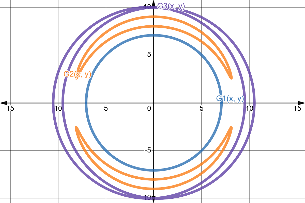
So the function \(G(x, y)\) representing the desired shape of our graph is:
\[\begin{align*} G(x,y)&=G_1(x,y) \cdot G_2(x,y) \cdot G_3(x,y) \\ &=\left(x^{2}+y^{2}-50\right)\left((y^{2}+x^{2}-8.5^{2})^{2}-(y^{2}-0.1x^{2})\right)\left((x^{2}+y^{2}-10^{2})^{2}-x^{2}\right) \end{align*}\]Combining the implicit equations
Once we have the background of the graph and the desired shape, we can combine both implicit equations through a reduction of loci to obtain the final graph \(M(x, y) = 0\). To combine the implicit equations \(F(x, y) = 0\) and \(G(x, y) = 0\), we apply the union property of loci:
\[M(x, y) = F(x, y) \cdot \frac{\sqrt{-G(x, y)}}{\sqrt{-G(x, y)}} = 0\]Substituting, we get this immense implicit equation:
\[M(x, y) = \cos\left(x+\cos\left(yx\right)-\sin\left(0.5x^{2}-y^{2}\right)\right)\ \frac{\sqrt{-\left(x^{2}+y^{2}-50\right)\left((y^{2}+x^{2}-8.5^{2})^{2}-(y^{2}-0.1x^{2})\right)\left((x^{2}+y^{2}-10^{2})^{2}-x^{2}\right)}}{\sqrt{-\left(x^{2}+y^{2}-50\right)\left((y^{2}+x^{2}-8.5^{2})^{2}-(y^{2}-0.1x^{2})\right)\left((x^{2}+y^{2}-10^{2})^{2}-x^{2}\right)}}=0\]whose locus is:
Conclusion
In this blog post we have explored the fascinating world of implicit equations and how they can be used to create surprising graphs. We learned that an implicit equation is a relation of the form \(F(x_1, \dots, x_n) = 0\), whose locus is its graph. We also saw that an implicit function is a function defined by an implicit equation, relating a dependent variable to the independent variables.
Along the way we analysed several properties of implicit equations that let us translate, expand, compress, reflect and combine loci, which gives us a wide range of possibilities for creating surprising graphs. We also saw how we can reduce loci by removing specific points, using techniques such as reduction by distinction and reduction by inequality.
Following a solid strategy, we proposed a series of steps for building our own surprising graph. These steps include defining the background of the graph, determining the desired shape, exploring and adjusting parameters, and combining implicit equations through reductions of loci.
Finally, we applied this strategy to build a fascinating graph, combining a background implicit equation with several implicit equations representing interesting shapes. Through experimentation and parameter tuning, we managed to create a surprising graph that stands out for its beauty and complexity.
In conclusion, we have shown that there is a lot to learn about implicit equations by playing with them, and that creativity and experimentation are key to discovering new ways of generating surprising graphs. So keep exploring and having fun with mathematics!
Bibliography
Lecture 24: Implicit Functions, Dartmouth College.
Álgebra y Geometría analítica, Universidad Tecnológica Nacional, Facultad Regional Buenos Aires.
Geometría III: Geometría analítica plana y del espacio, Elizabeth Vargas y Luis Núñez.